Introduction to PyFiberAmp
PyFiberAmp is a rate equation simulation library for rare-earth-doped fiber amplifiers and fiber lasers partly based on the Giles model [1].
With PyFiberAmp you can simulate:
- Both core-pumped and double-clad fiber amplifiers
- Simple continuous-wave, gain-switched and Q-switched fiber lasers
- Unlimited number of pump, signal and ASE channels
- Limited number of Raman channels
- Arbitrarily time-dependent beams from continuous-wave to nanosecond pulses
- Radially varying dopant concentration and excitation
- Automatically calculated Bessel, Gaussian and top-hat mode shapes
Additional benefits include:
- Built-in plotting commands: easy visualization of results
- Python interface: convenient for post-processing the data
- C++, Numba and Pythran backends: fast time-dynamic simulations
- Open source: see what’s happening under the hood
- Free of charge: install on as many computers as you like
Documentation is still in progress and available on Read the Docs. For practical examples, see the examples folder above. If you have a question, comment or feature request, please open a new issue on GitHub or contact me at pyfiberamp@gmail.com. If you find PyFiberAmp useful in your own project, I would also very much like to hear about it.
A visual example
Few-nanosecond pulses propagating in an Yb-doped fiber amplifier are distorted because of gain saturation. The Gaussian pulse with its exponential leading edge retains its shape better than the square or saw-tooth pulses.
Download
PyFiberAmp is not yet on PyPI. You can either download the code as a zip-file or clone the repository with
git clone git://github.com/Jomiri/pyfiberamp.git
and then install the library by executing
python setup.py install
in the (unzipped) download directory.
System requirements
PyFiberAmp depends on the standard scientific Python packages: Numpy, SciPy and Matplotlib and has been tested on Windows 7 and Windows 10. It should work on other operating systems as well provided that Python and the required packages are installed. The Anaconda distribution contains everything you’ll need out of the box.
Even though all of PyFiberAmp’s functionality is available in interpreted Python code, the use of one of the compiled backends (C++, Numba or Pythran) is recommended for computationally intensive time-dynamic simulations. The hand-written C++ extension is fastest but has also the strictest system requirements: Windows 7 or 10, Python 3.6 and a fairly modern CPU with AVX2 instruction support. The Pythran backend probably only works on Linux and requires that pythran is installed before installing PyFiberAmp. The Numba backend should work on all operating systems provided that Numba is available. Please open a new issue if you encounter problems with a backend that should work but does not.
Example
The simple example below demonstrates a core-pumped Yb-doped fiber amplifier. All units are in SI.
from pyfiberamp.steady_state import SteadyStateSimulation
from pyfiberamp.fibers import YbDopedFiber
yb_number_density = 2e25 # m^-3
core_radius = 3e-6 # m
length = 2.5 # m
core_na = 0.12
fiber = YbDopedFiber(length=length,
core_radius=core_radius,
ion_number_density=yb_number_density,
background_loss=0,
core_na=core_na)
simulation = SteadyStateSimulation()
simulation.fiber = fiber
simulation.add_cw_signal(wl=1035e-9, power=2e-3)
simulation.add_forward_pump(wl=976e-9, power=300e-3)
simulation.add_ase(wl_start=1000e-9, wl_end=1080e-9, n_bins=80)
result = simulation.run(tol=1e-5)
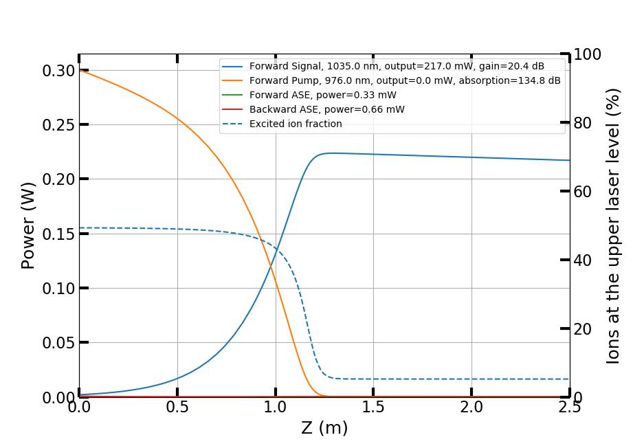
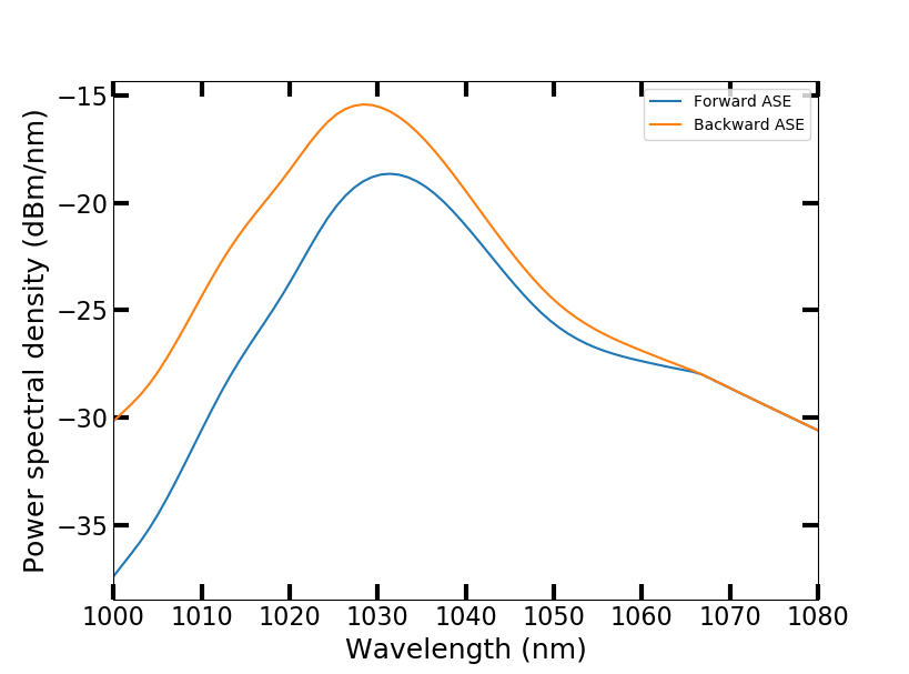
result.plot_amplifier_result()
The script calculates and plots the power evolution in the amplifier and the amplified spontaneous emission (ASE) spectra. The co-propagating pump is absorbed in the first ~1.2 m of the fiber while the signal experiences gain. When the pump has been depleted, the signal starts to be reabsorbed. ASE is stronger against the pumping direction.
For more usage examples, please see the Jupyter notebooks in the examples folder. More examples will be added in the future.
Fiber data
PyFiberAmp comes with spectroscopic data (effective absorption and emission cross sections) for Yb-doped germanosilicate fibers [3] and supports importing spectra for other dopants and glass compositions.
Theory basics
For a quick review on the theory, see the pyfiberamp theory.pdf file. Theory on the time-dynamic simulations is not yet included. A more complete description can be found in the references.
License
PyFiberAmp is licensed under the MIT license. The C++ extension depends on the pybind11 and Armadillo projects. See the license file for their respective licenses.
References
| [1] | C.R. Giles and E. Desurvire, “Modeling erbium-doped fiber amplifiers,” in Journal of Lightwave Technology, vol. 9, no. 2, pp. 271-283, Feb 1991. doi: 10.1109/50.65886 |
| [2] | R.G. Smith, “Optical Power Handling Capacity of Low Loss Optical Fibers as Determined by Stimulated Raman and Brillouin Scattering,” Appl. Opt. 11, 2489-2494 (1972) |
| [3] |
|